Geospatial data formats and metadata inspection

QGreenland Researcher Workshop 2023

Geospatial data formats

In general, we suggest formats that:

• Are non-proprietary
• Are broadly supported by common software tools
• Have rich metadata support

There are various data file formats for storing geospatial data and the selection of a format depends on use case and data type (raster vs vector).

The best formats for storing geospatial data have been designed for this purpose. Some general-purpose formats like CSV may be okay, but not great.

Finding information about formats

• Library of Congress list of digital formats
  • Check the “Licensing and patents” section to learn about openness of a format.
• Open Geospatial Consortium (OGC)-adopted standards
  • In these slides, 🌎 indicates an OGC-adopted standard.
• For information on other formats not covered in the following slides, please see our extra slides.

The OGC is a consortium that represents a large number of private and public organizations (including USGS, NOAA, Esri, AWS) with the goal to make geospatial data more “FAIR” (Findable, Accessible, Interoperable, and Reusable). More on this concept tomorrow!

We are only going to cover a few examples of common data formats in these slides. See our extra slides for more example formats.

Vector data formats

Microsoft .xls/.xlsx

• General-purpose
• Lacks metadata support
• No support for data types
• Proprietary (.xls)

GeoJSON 🌎

• One of OGC’s standard formats
• An extension of the JSON standard supporting geospatial metadata
• Text-based, can be read by humans

greenland-border.geojson

{
  "type":"FeatureCollection",
  "features":[
    {
      "type":"Feature",
      "id":"GRL",
      "properties":{"name":"Greenland"},
      "geometry":{
        "type":"Polygon",
        "coordinates":[[
          [-46.76379,82.62796],
          [-43.40644,83.22516],
          [-39.89753,83.18018],
          [-38.62214,83.54905],
          [-35.08787,83.64513],
          [-27.10046,83.51966],
          [-20.84539,82.72669],
          [-22.69182,82.34165],
          [-26.51753,82.29765],
          [-31.9,82.2],
          [-31.39646,82.02154],
          [-27.85666,82.13178],
          [-24.84448,81.78697],
          [-22.90328,82.09317],
          [-22.07175,81.73449],
          [-23.16961,81.15271],
          [-20.62363,81.52462],
          [-15.76818,81.91245],
          [-12.77018,81.71885],
          [-12.20855,81.29154],
          [-16.28533,80.58004],
          [-16.85,80.35],
          [-20.04624,80.17708],
          [-17.73035,80.12912],
          [-18.9,79.4],
          [-19.70499,78.75128],
          [-19.67353,77.63859],
          [-18.47285,76.98565],
          [-20.03503,76.94434],
          [-21.67944,76.62795],
          [-19.83407,76.09808],
          [-19.59896,75.24838],
          [-20.66818,75.15585],
          [-19.37281,74.29561],
          [-21.59422,74.22382],
          [-20.43454,73.81713],
          [-20.76234,73.46436],
          [-22.17221,73.30955],
          [-23.56593,73.30663],
          [-22.31311,72.62928],
          [-22.29954,72.18409],
          [-24.27834,72.59788],
          [-24.79296,72.3302],
          [-23.44296,72.08016],
          [-22.13281,71.46898],
          [-21.75356,70.66369],
          [-23.53603,70.471],
          [-24.30702,70.85649],
          [-25.54341,71.43094],
          [-25.20135,70.75226],
          [-26.36276,70.22646],
          [-23.72742,70.18401],
          [-22.34902,70.12946],
          [-25.02927,69.2588],
          [-27.74737,68.47046],
          [-30.67371,68.12503],
          [-31.77665,68.12078],
          [-32.81105,67.73547],
          [-34.20196,66.67974],
          [-36.35284,65.9789],
          [-37.04378,65.93768],
          [-38.37505,65.69213],
          [-39.81222,65.45848],
          [-40.66899,64.83997],
          [-40.68281,64.13902],
          [-41.1887,63.48246],
          [-42.81938,62.68233],
          [-42.41666,61.90093],
          [-42.86619,61.07404],
          [-43.3784,60.09772],
          [-44.7875,60.03676],
          [-46.26364,60.85328],
          [-48.26294,60.85843],
          [-49.23308,61.40681],
          [-49.90039,62.38336],
          [-51.63325,63.62691],
          [-52.14014,64.27842],
          [-52.27659,65.1767],
          [-53.66166,66.09957],
          [-53.30161,66.8365],
          [-53.96911,67.18899],
          [-52.9804,68.35759],
          [-51.47536,68.72958],
          [-51.08041,69.14781],
          [-50.87122,69.9291],
          [-52.013585,69.574925],
          [-52.55792,69.42616],
          [-53.45629,69.283625],
          [-54.68336,69.61003],
          [-54.75001,70.28932],
          [-54.35884,70.821315],
          [-53.431315,70.835755],
          [-51.39014,70.56978],
          [-53.10937,71.20485],
          [-54.00422,71.54719],
          [-55,71.406537],
          [-55.83468,71.65444],
          [-54.71819,72.58625],
          [-55.32634,72.95861],
          [-56.12003,73.64977],
          [-57.32363,74.71026],
          [-58.59679,75.09861],
          [-58.58516,75.51727],
          [-61.26861,76.10238],
          [-63.39165,76.1752],
          [-66.06427,76.13486],
          [-68.50438,76.06141],
          [-69.66485,76.37975],
          [-71.40257,77.00857],
          [-68.77671,77.32312],
          [-66.76397,77.37595],
          [-71.04293,77.63595],
          [-73.297,78.04419],
          [-73.15938,78.43271],
          [-69.37345,78.91388],
          [-65.7107,79.39436],
          [-65.3239,79.75814],
          [-68.02298,80.11721],
          [-67.15129,80.51582],
          [-63.68925,81.21396],
          [-62.23444,81.3211],
          [-62.65116,81.77042],
          [-60.28249,82.03363],
          [-57.20744,82.19074],
          [-54.13442,82.19962],
          [-53.04328,81.88833],
          [-50.39061,82.43883],
          [-48.00386,82.06481],
          [-46.59984,81.985945],
          [-44.523,81.6607],
          [-46.9007,82.19979],
          [-46.76379,82.62796],
        ]],
      },
    },
  ],
}

Two examples of vector data formats, one is less-suited for the task than the other. If you’re looking for more examples, please find the “extra” slide deck for this module on the workshop website.

Microsoft Excel formatted data is common but suffers from some drawbacks.

Prefer something like GeoJSON instead, which is an adopted OGC standard and supports CRS metadata.

• XLS/XLSX:
  • No support for data types: “The display of stored numbers as integers or currency is through display format options.”
  • XLSX is an “open” extension of XML.
  • Like CSV, has no standard metadata support.

Raster data formats

ESRI ASCII Grid

• Text-based, can be read by humans
• Limited metadata support: CRS and measurement-related information cannot be stored in the file alongside the data.

$ cat example_data.asc 

ncols         5
nrows         3
xllcorner     -30.0
yllcorner     75.0
cellsize      10.183314
NODATA_value  -9999
100 -9999 7 3 -9999
-9999 14 5 0 1
-9999 11 23 12 -9999

GeoTIFF 🌎

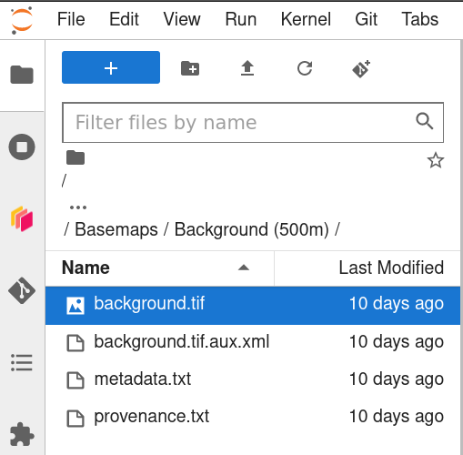
• Raster data
• An extension of the TIFF standard supporting geospatial metadata
• Works with almost all image viewer software

QGreenland’s raster datasets are stored as GeoTiffs

Two examples of raster data formats. ESRI ASCII Grid format is human readable and widely supported but has limited metadata support.

GeoTIFFs are OGC standard data formats.

Flexible data formats

Examples of modern data formats that are open, interoperable, and have rich metadata support include NetCDF and GeoPackage.

NetCDF 🌎

• Raster (and vector) data
• Extension of HDF5 🌎
• Self-Describing
• Efficient storage of multi-dimensional arrays of data (e.g., time, elevation, longitude, latitude as dimensions of a temperature variable)
• NetCDF Climate and Forecast (CF) Metadata Conventions are widely adopted in the science community.

GeoPackage 🌎

• Raster, vector, and more…
• A specialized SQLite database supporting geospatial metadata
• Can store datasets of different types in a single file
• QGreenland’s vector datasets are stored as GeoPackages.

Inspecting Data

What tool should I use?

The best one for the job! Explore the alternatives available in the ecosystem you want to work!

• GUI-based GIS tools (QGIS!) are useful for visualization of data, especially in comparison with other layers like a basemap.
• Command-line tools are especially useful for getting a quick answer.
• Language-specific (e.g., Python) tools are good for automations or research code.
  • QGIS has a Python API!

QGIS Layer Properties

CRS of a QGreenland layer

Remember that once you have added data as a layer in QGIS, you can inspect it’s metadata via the Information tab in the layer’s Properties window.

Make sure to double-check the CRS of the data you are looking at matches the other layers you want to compare it to! Remember that differences between e.g., the datum can be significant!

CLI Tools

We are going to focus on the GDAL/OGR command-line tools.

• GDAL/OGR underlie many of the raster and vector data processing functions in QGIS.
• Also utilized by many python-based geospatial libraries like rasterio and shapely.

• “OGR” used to stand for “OpenGIS Simple Features Reference Implementation” but is now the name is “OGR Simple Features Library”. “OGR” is left for historical reasons. OSGeo GDAL FAQ

Learning more about CLI tools

The first thing to try is <command> --help:

gdalinfo --help

Usage: gdalinfo [--help-general] [-json] [-mm] [-stats] [-hist] [-nogcp] [-nomd]
                [-norat] [-noct] [-nofl] [-checksum] [-proj4]
                [-listmdd] [-mdd domain|`all`] [-wkt_format WKT1|WKT2|...]*
                [-sd subdataset] [-oo NAME=VALUE]* datasetname

Learning more about CLI tools (man)

If the --help output is not useful, try the “manual pages” with the man command.

man gdalinfo

gdalinfo(1)            General Commands Manual            gdalinfo(1)

NAME
       gdalinfoLists information about a raster dataset.

SYNOPSIS
       gdalinfo [--help-general] [-json] [-mm] [-stats] [-hist] [-nogcp] [-nomd]
                [-norat] [-noct] [-nofl] [-checksum] [-proj4]
                [-listmdd] [-mdd domain|`all`]* [-wkt_format WKT1|WKT2|...]
                [-sd subdataset] [-oo NAME=VALUE]* datasetname

DESCRIPTION
       The gdalinfo program lists various information about a GDAL
       supported raster dataset.

       -json
           Display the output in json format.

       -mm
           Force computation of the actual min/max values for each
           band in the dataset.

       -stats
           Read and display image statistics. Force computation if no
           statistics are stored in an image.

       -approx_stats
           Read and display image statistics. Force computation if no
           statistics are stored in an image. However, they may be
           computed based on overviews or a subset of all tiles.
           Useful if you are in a hurry and don't want precise stats.

       -hist
           Report histogram information for all bands.

       -nogcp
           Suppress ground control points list printing. It may be
           useful for datasets with huge amount of GCPs, such as L1B
           AVHRR or HDF4 MODIS which contain thousands of them.

       -nomd
           Suppress metadata printing. Some datasets may contain a
           lot of metadata strings.

       -norat
           Suppress printing of raster attribute table.

       -noct
           Suppress printing of color table.

       -checksum
           Force computation of the checksum for each band in the
           dataset.

       -listmdd
           (GDAL >= 1.11) List all metadata domains available for the
           dataset.

       -mdd domain
           Report metadata for the specified domain. Starting with
           GDAL 1.11, 'all' can be used to report metadata in all
           domains

       -nofl
           (GDAL >= 1.9.0) Only display the first file of the file
           list.

       -wkt_format WKT1/WKT2/...
           (GDAL >= 3.0.0) WKT format used to display the SRS.
           Currently supported values are: WKT1, WKT2 (latest WKT
           version, currently WKT2_2018), WKT2_2015, WKT2_2018

       -sd subdataset
           (GDAL >= 1.9.0) If the input dataset contains several
           subdatasets read and display a subdataset with specified
           number (starting from 1). This is an alternative of giving
           the full subdataset name.

       -proj4
           (GDAL >= 1.9.0) Report a PROJ.4 string corresponding to
           the file's coordinate system.

       -oo NAME=VALUE:
           (starting with GDAL 2.0) Dataset open option (format
           specific)

       The gdalinfo will report all of the following (if known):

       • The format driver used to access the file.
       • Raster size (in pixels and lines).
       • The coordinate system for the file (in OGC WKT).
       • The geotransform associated with the file (rotational
         coefficients are currently not reported).
       • Corner coordinates in georeferenced, and if possible
         lat/long based on the full geotransform (but not GCPs).
       • Ground control points.
       • File wide (including subdatasets) metadata.
       • Band data types.
       • Band color interpretations.
       • Band block size.
       • Band descriptions.
       • Band min/max values (internally known and possibly
         computed).
       • Band checksum (if computation asked).
       • Band NODATA value.
       • Band overview resolutions available.
       • Band unit type (i.e.. 'meters' or 'feet' for elevation
         bands).
       • Band pseudo-color tables.
C API
       Starting with GDAL 2.1, this utility is also callable from C
       with GDALInfo().
EXAMPLE
       gdalinfo ~/openev/utm.tif
       Driver: GTiff/GeoTIFF
       Size is 512, 512
       Coordinate System is:
       PROJCS["NAD27 / UTM zone 11N",
           GEOGCS["NAD27",
               DATUM["North_American_Datum_1927",
                   SPHEROID["Clarke 1866",6378206.4,294.978698213901]],
               PRIMEM["Greenwich",0],
               UNIT["degree",0.0174532925199433]],
           PROJECTION["Transverse_Mercator"],
           PARAMETER["latitude_of_origin",0],
           PARAMETER["central_meridian",-117],
           PARAMETER["scale_factor",0.9996],
           PARAMETER["false_easting",500000],
           PARAMETER["false_northing",0],
           UNIT["metre",1]]
       Origin = (440720.000000,3751320.000000)
       Pixel Size = (60.000000,-60.000000)
       Corner Coordinates:
       Upper Left  (  440720.000, 3751320.000) (117d38'28.21"W, 33d54'8.47"N)
       Lower Left  (  440720.000, 3720600.000) (117d38'20.79"W, 33d37'31.04"N)
       Upper Right (  471440.000, 3751320.000) (117d18'32.07"W, 33d54'13.08"N)
       Lower Right (  471440.000, 3720600.000) (117d18'28.50"W, 33d37'35.61"N)
       Center      (  456080.000, 3735960.000) (117d28'27.39"W, 33d45'52.46"N)
       Band 1 Block=512x16 Type=Byte, ColorInterp=Gray
AUTHORS
       Frank Warmerdam warmerdam@pobox.com, Silke Reimer
       silke@intevation.de

GDAL                       Sun Mar 29 2020                gdalinfo(1)

If you still get stuck, check for official documentation pages online, forums (e.g., stackoverflow) that cater to technical questions, and tutorials provided by research/educational organizations.

Raster data inspection: gdalinfo

gdalinfo bedmachine_bed.tif

Driver: GTiff/GeoTIFF
Files: bedmachine_bed.tif
       bedmachine_bed.tif.aux.xml
Size is 14844, 21876
Coordinate System is:
PROJCRS["WGS 84 / NSIDC Sea Ice Polar Stereographic North",
    BASEGEOGCRS["WGS 84",
        DATUM["World Geodetic System 1984",
            ELLIPSOID["WGS 84",6378137,298.257223563,
                LENGTHUNIT["metre",1]]],
        PRIMEM["Greenwich",0,
            ANGLEUNIT["degree",0.0174532925199433]],
        ID["EPSG",4326]],
    CONVERSION["US NSIDC Sea Ice polar stereographic north",
        METHOD["Polar Stereographic (variant B)",
            ID["EPSG",9829]],
        PARAMETER["Latitude of standard parallel",70,
            ANGLEUNIT["degree",0.0174532925199433],
            ID["EPSG",8832]],
        PARAMETER["Longitude of origin",-45,
            ANGLEUNIT["degree",0.0174532925199433],
            ID["EPSG",8833]],
        PARAMETER["False easting",0,
            LENGTHUNIT["metre",1],
            ID["EPSG",8806]],
        PARAMETER["False northing",0,
            LENGTHUNIT["metre",1],
            ID["EPSG",8807]]],
    CS[Cartesian,2],
        AXIS["easting (X)",south,
            MERIDIAN[45,
                ANGLEUNIT["degree",0.0174532925199433]],
            ORDER[1],
            LENGTHUNIT["metre",1]],
        AXIS["northing (Y)",south,
            MERIDIAN[135,
                ANGLEUNIT["degree",0.0174532925199433]],
            ORDER[2],
            LENGTHUNIT["metre",1]],
    USAGE[
        SCOPE["unknown"],
        AREA["World - N hemisphere - north of 60°N"],
        BBOX[60,-180,90,180]],
    ID["EPSG",3413]]
Data axis to CRS axis mapping: 1,2
Origin = (-997978.940007228753529,-329743.070899212907534)
Pixel Size = (149.996827426226332,-149.996827426226389)
Metadata:
  AREA_OR_POINT=Area
  bed#grid_mapping=mapping
  bed#long_name=bed topography
  bed#source=Mass conservation (Mathieu Morlighem)
  bed#standard_name=bedrock_altitude
  bed#units=meters
  bed#_FillValue=-9999
  mapping#false_easting=0
  mapping#false_northing=0
  mapping#geoid=eigen-6c4
  mapping#grid_mapping_name=polar_stereographic
  mapping#inverse_flattening=298.2794050428205
  mapping#latitude_of_projection_origin=90
  mapping#semi_major_axis=6378273
  mapping#standard_parallel=70
  mapping#straight_vertical_longitude_from_pole=-45
  NC_GLOBAL#Author=Mathieu Morlighem
  NC_GLOBAL#Conventions=CF-1.7
  NC_GLOBAL#Data_citation=Morlighem M. et al., (2017), BedMachine v3: Complete bed topography and ocean bathymetry mapping of Greenland from multi-beam echo sounding combined with mass conservation, Geophys. Res. Lett., 44, doi:10.1002/2017GL074954. (http://onlinelibrary.wiley.com/doi/10.1002/2017GL074954/full)
  NC_GLOBAL#ice_density (kg m-3)=917
  NC_GLOBAL#license=No restrictions on access or use
  NC_GLOBAL#no_data=-9999
  NC_GLOBAL#nx=10218
  NC_GLOBAL#ny=18346
  NC_GLOBAL#proj4=+init=epsg:3413
  NC_GLOBAL#Projection=Polar Stereographic North (70N, 45W)
  NC_GLOBAL#sea_water_density (kg m-3)=1023
  NC_GLOBAL#spacing=150
  NC_GLOBAL#Title=BedMachine Greenland
  NC_GLOBAL#version=20-Apr-2021 (v4.10)
  NC_GLOBAL#xmin=-652925
  NC_GLOBAL#ymax=-632675
  x#long_name=Cartesian x-coordinate
  x#standard_name=projection_x_coordinate
  x#units=meter
  y#long_name=Cartesian y-coordinate
  y#standard_name=projection_y_coordinate
  y#units=meter
Image Structure Metadata:
  COMPRESSION=DEFLATE
  INTERLEAVE=BAND
Corner Coordinates:
Upper Left  ( -997978.940, -329743.071) (116d42'57.18"W, 80d19'10.86"N)
Lower Left  ( -997978.940,-3611073.668) ( 60d26'56.41"W, 56d22'33.59"N)
Upper Right ( 1228573.966, -329743.071) ( 29d58'34.22"E, 78d17'47.47"N)
Lower Right ( 1228573.966,-3611073.668) ( 26d12'37.67"W, 55d48' 2.10"N)
Center      (  115297.513,-1970408.369) ( 41d39' 4.26"W, 71d55'29.45"N)
Band 1 Block=256x256 Type=Float32, ColorInterp=Gray
  Min=-5571.673 Max=3672.355
  Minimum=-5571.673, Maximum=3672.355, Mean=-307.314, StdDev=1161.000
  NoData Value=-9999
  Overviews: 7422x10938, 3711x5469, 1856x2735, 928x1368
  Unit Type: meters
  Metadata:
    grid_mapping=mapping
    long_name=bed topography
    NETCDF_VARNAME=bed
    source=Mass conservation (Mathieu Morlighem)
    standard_name=bedrock_altitude
    STATISTICS_MAXIMUM=3672.35546875
    STATISTICS_MEAN=-307.31420082049
    STATISTICS_MINIMUM=-5571.6728515625
    STATISTICS_STDDEV=1160.9999064556
    STATISTICS_VALID_PERCENT=57.73
    units=meters
    _FillValue=-9999

Using gdalinfo to inspect the metadata in a GeoTiff.

Highlighted information, in order:

• Driver & associated files
• Grid size, in “pixels”
• Well-Known Text represents CRS with hierarchical data, which gdalinfo nicely indents for us.
• The “top-level” EPSG is shown as 3413.
• Pixel size, in projected units
• Global metadata: These are metadata that were included in the original NetCDF source dataset. We will discuss more about this pitfall in the “Transformations” module.
• Band information
  • NoData value
  • Overviews: Various down-sampled versions of the data for performance when zoomed out.
  • Units
  • metadata

Vector data inspection: ogrinfo

ogrinfo -al -so populated_places.gpkg

INFO: Open of `populated_places.gpkg'
      using driver `GPKG' successful.

Layer name: SELECT
Geometry: Point
Feature Count: 83
Extent: (-605594.054592, -3322344.525361) - (837631.269958, -1140855.537211)
Layer SRS WKT:
PROJCRS["WGS 84 / NSIDC Sea Ice Polar Stereographic North",
    BASEGEOGCRS["WGS 84",
        ENSEMBLE["World Geodetic System 1984 ensemble",
            MEMBER["World Geodetic System 1984 (Transit)"],
            MEMBER["World Geodetic System 1984 (G730)"],
            MEMBER["World Geodetic System 1984 (G873)"],
            MEMBER["World Geodetic System 1984 (G1150)"],
            MEMBER["World Geodetic System 1984 (G1674)"],
            MEMBER["World Geodetic System 1984 (G1762)"],
            MEMBER["World Geodetic System 1984 (G2139)"],
            ELLIPSOID["WGS 84",6378137,298.257223563,
                LENGTHUNIT["metre",1]],
            ENSEMBLEACCURACY[2.0]],
        PRIMEM["Greenwich",0,
            ANGLEUNIT["degree",0.0174532925199433]],
        ID["EPSG",4326]],
    CONVERSION["US NSIDC Sea Ice polar stereographic north",
        METHOD["Polar Stereographic (variant B)",
            ID["EPSG",9829]],
        PARAMETER["Latitude of standard parallel",70,
            ANGLEUNIT["degree",0.0174532925199433],
            ID["EPSG",8832]],
        PARAMETER["Longitude of origin",-45,
            ANGLEUNIT["degree",0.0174532925199433],
            ID["EPSG",8833]],
        PARAMETER["False easting",0,
            LENGTHUNIT["metre",1],
            ID["EPSG",8806]],
        PARAMETER["False northing",0,
            LENGTHUNIT["metre",1],
            ID["EPSG",8807]]],
    CS[Cartesian,2],
        AXIS["easting (X)",south,
            MERIDIAN[45,
                ANGLEUNIT["degree",0.0174532925199433]],
            ORDER[1],
            LENGTHUNIT["metre",1]],
        AXIS["northing (Y)",south,
            MERIDIAN[135,
                ANGLEUNIT["degree",0.0174532925199433]],
            ORDER[2],
            LENGTHUNIT["metre",1]],
    USAGE[
        SCOPE["Polar research."],
        AREA["Northern hemisphere - north of 60°N onshore and offshore, including Arctic."],
        BBOX[60,-180,90,180]],
    ID["EPSG",3413]]
Data axis to CRS axis mapping: 1,2
FID Column = fid
Geometry Column = geom
ID: Integer64 (0.0)
New Greenlandic: String (0.0)
Old Greenlandic: String (0.0)
Danish: String (0.0)
Alternative placename: String (0.0)
Object designation: String (0.0)
Source: String (0.0)
Municipality: String (0.0)
Notes: String (0.0)
Date of registration: String (0.0)
Modification date: String (0.0)
Authorized: String (0.0)
Authorized date: String (0.0)
Project manager: String (0.0)
KMS_id: String (0.0)
Latitude: Real (0.0)
Longitude: Real (0.0)
Card: String (0.0)
Namer: String (0.0)
Namesake: String (0.0)
Meaning of the placename: String (0.0)
Placename history: String (0.0)
Danish explanation of Object designation: String (0.0)
Greenlandic explanation of Object designation: String (0.0)
English explanation of Object designation: String (0.0)
Translation notes: String (0.0)
label: String (0.0)

• -al: All layers
• -so: Summary only; don’t list individual features.

Highlights, in order:

• Info on the driver used to open this GeoPackage.
• There may be many layers, but this particular GeoPackage has only one called “SELECT”, which is a poor name.
• This layer is a Point layer.
• 83 points.
• Spatial extent
• Like gdalinfo, the CRS is in WKT.
• The “top-level” EPSG code.
• These are attribute table columns and their datatypes.

Missing metadata??

Please note: This dataset was intentionally modified to remove metadata. This example does not reflect the quality of the original dataset.

gdalinfo content/examples/data-scenarios/missing-metadata/dem_without_metadata.tif

Driver: GTiff/GeoTIFF
Files: dem_without_metadata.tif
Size is 301, 561
Metadata:
  TIFFTAG_XRESOLUTION=1
  TIFFTAG_YRESOLUTION=1
Image Structure Metadata:
  INTERLEAVE=BAND
Corner Coordinates:
Upper Left  (    0.0,    0.0)
Lower Left  (    0.0,  561.0)
Upper Right (  301.0,    0.0)
Lower Right (  301.0,  561.0)
Center      (  150.5,  280.5)
Band 1 Block=301x6 Type=Float32, ColorInterp=Gray

No Coordinate Reference System is specified!

Sometimes we want to work with data that has limited or no metadata! This is an example of what such a situation might look like. We will talk more about how to handle situations like this in an upcoming module.

• Corner coordinates are in grid space.
  • NOTE: the upper-left corner coordinates are (0, 0); this is a red flag that the data is not properly geolocated.
• There is no WKT or other specification of a coordinate reference system.

Additional resources

More examples of common data formats and methods of inspecting data are in the Additional slides: Geospatial Data Formats and Inspection.

Exercise

💪 Data inspection with JupyterLab